Introduction
Here’s the scenario: I’m working on my project, using a git repo to track changes. I’m excited about the project or a certain result, and I’d like to tell everyone about it by making a blog post with blogdown.
But how do I utilize all the work I’ve already done in the project? I’ve curated the data, built the plots, and saved my complicated analysis as a .RDS file. I’d like to reuse that work, and as a one forum user put it “copying rmarkdown files is a nonstarter.”
Inspired by this discussion on the R Studio forum, I’d like to share my workflow that I use to blog about my projects with Hugo/blogdown/Netlify. We’ll look at
- git submodules
- knitr working directories
- knitr code externalization
I’ll demonstrate this workflow by example. This Github repo will be the external project we’d like to blog about. And this very post is where we’d like to do it. This means you should also follow the .Rmd for this post found on my website’s Github repo.
git Setup
For our purposes, we’ll assume your project repo exists on Github. If you don’t feel comfortable with command line git clone/pull/add/commit/push, I strongly recommend Jenny Bryan’s bookdown on git for R users. The tutorial will teach you the basics of working with git locally and on Github.
The purpose of the submodule is to make the contents of your project easily available and accessible. We want your .Rmd posts to utilize all the data and functions without copy/pasting. And we want to maintain version control and a connection to the project’s origin/master so you can incorporate updates.
For me, git submodules are preferable to other local clones of your project’s Github repo. First, I like organizing the projects my blog uses within the website’s directory structure. Second, submodules have an added layer of version control that handles project updates in a careful way. This helps to avoid breaking my posts due to a project update.
Creating
All my blog posts live here:
website2/content/blogI like creating a sub-directory that will hold the submodules for any project:
website2/content/blog/external_dataThen we can create the submodule with the submodule command:
Timothys-MacBook-Pro:external_data Tim$ git submodule add https://github.com/tmastny/git-blogdown-workflow.git
Cloning into '/Users/Tim/website2/content/blog/external_data/git-blogdown-workflow'...
remote: Counting objects: 10, done.
remote: Compressing objects: 100% (7/7), done.
remote: Total 10 (delta 0), reused 7 (delta 0), pack-reused 0
Unpacking objects: 100% (10/10), done.
When we git add/commit/push the changes to the website2 repo you’ll notice that the folder icon has changed. This indicates that website’s repo is now tracking the project’s repo at a certain commit, rather than a copy of those files at a moment in time.
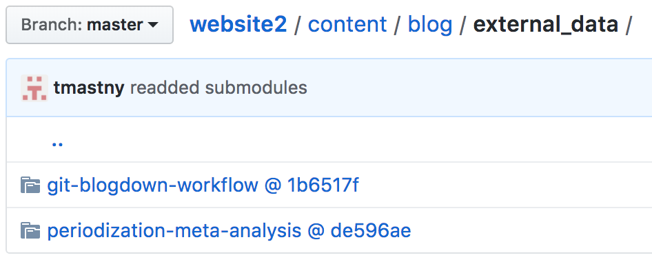
In fact, if you click the folder you will be taken to the git-blogdown-workflow Github repo. This is exactly what we want. Instead of a static copy of the project’s file, we have a version controlled copy that is linked to the project’s Github repo.
Lastly, you should also edit your config.toml file to ignore your external_data folder, or where ever you plan to put your submodules.
ignoreFiles = ["\\.Rmd$", "_files$", "_cache$",
               "blogdown$", "external_data$"]
Since Hugo can’t build .Rmd files, blogdown compiles your .Rmd to .html. These .html files include all the necessary data, so there is no reason for Hugo to copy the submodules to the public/ directory.
Updating and Version Control
On a normal git repo, to receive the latest changes to your local branch you use git pull. But git pull only brings in changes to the top level git repo, which is the website’s repo. This is by design.
Imagine you write a post that includes content from a project submodule. Months later a teammate changes a feature your blog post depends on. If the submodule was updated automatically with pull your blog posts could break unexpectedly.
Therefore, to avoid unexpected conflicts we need to explicitly receive updates from submodules.
The first method is to navigate to the submodule and use git fetch/merge. For example,
Timothys-MacBook-Pro:blog Tim$ cd git-blogdown-workflow/
Timothys-MacBook-Pro:git-blogdown-workflow Tim$ git fetch
remote: Counting objects: 3, done.
remote: Compressing objects: 100% (2/2), done.
remote: Total 3 (delta 1), reused 3 (delta 1), pack-reused 0
Unpacking objects: 100% (3/3), done.
From https://github.com/tmastny/git-blogdown-workflow
   3149843..e207121  master     -> origin/master
Timothys-MacBook-Pro:git-blogdown-workflow Tim$ git merge origin/master
Updating 3149843..e207121
Fast-forward
 plot_model.R | 10 ++++++++++
 1 file changed, 10 insertions(+)
 create mode 100644 plot_model.R
Note that git pull, the shortcut for git fetch/merge used on normal git repos does not work for submodules.
Or if you want to update all your submodules, you can use the shortcut git submodule update --remote:
Timothys-MacBook-Pro:blog Tim$ git submodule update --remote
Submodule path 'git-blogdown-workflow': checked out 'ce0d3a2f200eac6cd2a2980110137f7917e30b1d'
remote: Counting objects: 6, done.
remote: Compressing objects: 100% (4/4), done.
remote: Total 6 (delta 3), reused 5 (delta 2), pack-reused 0
Unpacking objects: 100% (6/6), done.
From https://github.com/tmastny/periodization-meta-analysis
   b29483b..de596ae  master     -> origin/master
Submodule path 'periodization-meta-analysis': checked out 'de596aed6a5535f7f4cdd270644e7993625b3f78'
But remember, pulling unexpected changes from your submodules can break your blog posts.
Code Externalization by Chunks
Now our blog posts lives in
website2/content/blogand we have a project submodule here:
website2/content/blog/external_data/git-blogdown-workflowBy default knitr assumes that the root directory is the one that the .Rmd lives in, so in this case blog/. However, we’d like our blog post to execute code that thinks its root is git-blogdown-workflow/.
We can change this default behavior in the setup chunk of the .Rmd with knitr::opts_knit$set(root.dir = ...). For example, here is the setup chunk I have in the beginning of this blog post:
```{r setup, include=FALSE}
knitr::opts_chunk$set(echo = TRUE, warning=FALSE, message=FALSE,
                      results='show', cache=FALSE, autodep=FALSE)
knitr::opts_knit$set(root.dir = 'external_data/git-blogdown-workflow/')
```
Note that I strongly recommend setting cache and autodep to false in the chunk options. In my experience, reading in external data can confuse the cache resulting in data existing where it shouldn’t. And if you want to use the cache because the blog post is doing a lot of expensive calculations, I recommend moving that code into a .R script within the project. Then you can save the results as .RDS file, which you can read into your blog post.
Now that our .Rmd thinks it lives in the project directory git-blogdown-workflow, we can start using the project’s files.
Here are the two most common procedures. First, to utilize external .R scripts within the blog post’s .Rmd we need to use knitr::read_chunk.
```{r}
knitr::read_chunk(path = 'your_script.R')
```
This will initialize the script within the blog’s .Rmd environment and allow us to call the code chunks.
In the .R script, code chunks will be delimited by this decoration:
## ---- chunk_name ----To call that chunk within the .Rmd session of this blog, we need to do the following:
```{r chunk_name}
```
That will execute the chunk within this session. The results will also be available to use within the blog’s .Rmd environment.
Let’s work through an example.
Example 1: The Basics
We’ll start simple by working with the R script sim.R.
Before we can call the chunks in our file, we need to initialize the .R script with read_chunk.1
```{r}
knitr::read_chunk(path = 'sim.R')
```
knitr::read_chunk(path = 'sim.R')This does not execute the code, but allows your blog post’s .Rmd environment to utilize chunks from that .R script.
After we’ve initialized the script with read_chunk, we can now call the code via the code externalization decorators we’ve added to the source code of sim.R. For example,
```{r simulate_function}
```
which produces
library(tidyverse)
library(magrittr)

monty_hall_sim <- function (door, switch) {
  doors <- c('a', 'b', 'c')
  prize <- sample(doors, size = 1)
  open_door <- sample(setdiff(doors, c(prize, door)), size = 1)
  if (switch) {
    door <- setdiff(doors, c(door, open_door))
  }
  return(door == prize)
}
This helps with portability and maintainability. We haven’t copied any code or scripts. The project script sim.R is being pull from the repo, so if the file is modified there, it will be modified here as well.
And another useful feature is that calling simulate_function evaluates the code in the .Rmd environment of the blog post. So we can use the function within the post!
monty_hall_sim('a', TRUE)## [1] TRUEThis is nice. We can easily add simple, exploratory examples to the blog post that we wouldn’t want cluttering the .R script.
Let’s call the next chunk:
```{r run_simulation}
```
d <- tibble(
door = sample(c('a', 'b', 'c'), size = 1000, replace = TRUE),
switch = sample(c(TRUE, FALSE), size = 1000, replace = TRUE)
)
d %<>%
mutate(prize = mapply(monty_hall_sim, door, switch))Now we have the tibble d in our blog environment. For example, we can show
head(d)## # A tibble: 6 x 3
## door switch prize
## <chr> <lgl> <lgl>
## 1 c F F
## 2 b T T
## 3 c F F
## 4 b T T
## 5 a F F
## 6 c T FYou do need to be careful with this data. Any future chunks you call from sim.R evaluate the code in the current environment. So if d were gone, the next chunk would fail:
a <- d
d <- NULL
```{r plot_results}
```d %>%
group_by(switch) %>%
mutate(attempt = row_number()) %>%
mutate(success_ratio = cumsum(prize)/attempt) %>%
ungroup() %>%
ggplot() +
geom_line(aes(x = attempt, y = success_ratio, color = switch))## Error in UseMethod("group_by_"): no applicable method for 'group_by_' applied to an object of class "NULL"So you need to make sure you don’t change the environmental variables in a way future chunks don’t except. A good rule of thumb is to not change or make new variables within the blog environment. Only explore and view objects created from the chunks.
Let’s fix our mistake and call the plot chunk again.
d <- a```{r plot_results}
```d %>%
group_by(switch) %>%
mutate(attempt = row_number()) %>%
mutate(success_ratio = cumsum(prize)/attempt) %>%
ungroup() %>%
ggplot() +
geom_line(aes(x = attempt, y = success_ratio, color = switch))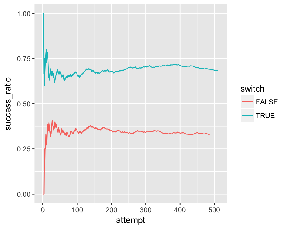
Example 2: External Data
The last example was nice, but a little unrealistic. Usually we use R to work with external data.
Again, we’ll do this by example. This time we want to showcase fit_model.R.
knitr::read_chunk('fit_model.R')This script fits a linear model to tidied_periodization.csv2 and plots the results.
Let’s try the first chunk:
```{r read_data}
```
d <- read_csv(file = 'tidied_periodization.csv')Even though our blog post’s .Rmd is actually in the directory above tidied_periodization.csv, we can read file as if the .Rmd was in the project’s directory. This is because we changed the root directory in our setup chunk.
The next two chunks involve fitting and saving a linear model.
# copied from fit_model.R for reference
## ---- fit_model ----
m <- lm(post ~ pre, data = d)

## ---- save_fit ----
saveRDS(m, file = 'saved_model.rds')
Often we’d like to show how to fit the model, but we don’t want to do the computation in the blog post. For me, writing a blog post is 90% rewriting and reorganizing. Waiting to fit models is very disruptive, especially when working with machine learning algorithms or Bayesian packages such as brms or rstan that take a very long time to fit.
There is a straightforward way work-around. First we call the fit_model chunk without evaluating it, so we can show how to fit the model.
```{r fit_model, eval=FALSE}
```
m <- lm(post ~ pre, data = d)Next, we load the model from the .RDS file within the project, with echo=FALSE so it doesn’t disrupt the narrative of the post.
```{r, echo=FALSE}
m <- readRDS('saved_model.rds')
```
And even though we haven’t executed fit_model.R linearly, we can still execute the final chunk because we’ve read in the model:
```{r plot_model}
```
d %>%
mutate(pred = predict(m, newdata = .)) %>%
ggplot(aes(x = pre)) +
geom_point(aes(y = post)) +
geom_line(aes(y = pred)) +
xlim(0, 420) + ylim(0, 500)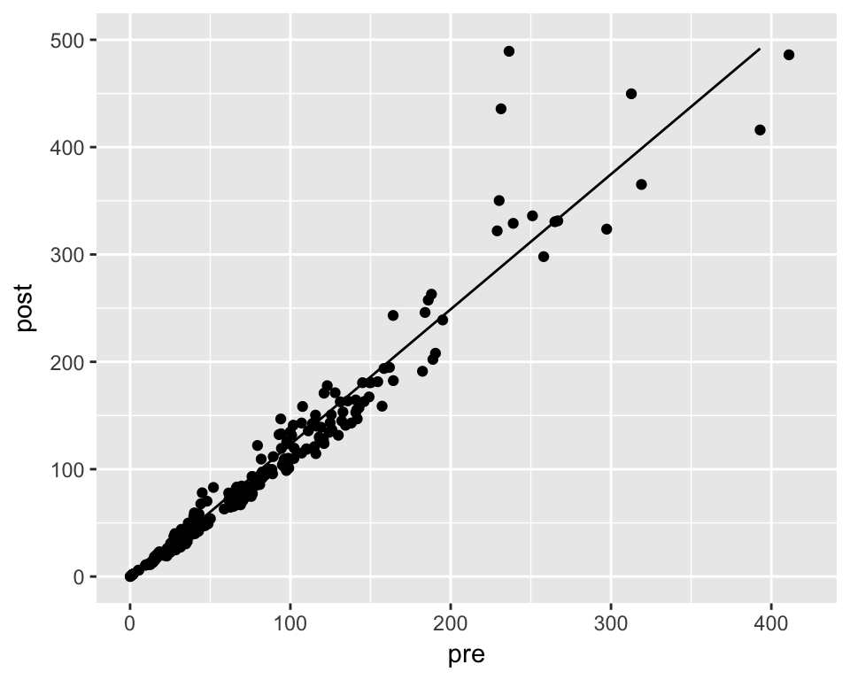
Conclusion
The key takeaway is that we can make our .Rmd file think that it exists in our project directory by calling
knitr::opts_knit$set(root.dir = ...)And with code externalization, you can interactively execute your source code to blog about your methods, or to share your final results.
I also think project submodules are a natural way to organize your work within your blog or website’s repo, as opposed to symbolic links which are more invisible and can change between operating systems.
I would also like to point out that personal R packages, as described by Hilary Parker and others, is another way to make personal projects more reusable and shareable. However, for small projects I think there is still a lot of overhead for creating packages (especially when trying to manage dependencies). Likewise, I’m not sure how to easily utilize the source code with read_chunk on an installed package. Therefore I’m not convinced they are the right tool for the job here.
Acknowledgements
Thanks to Yihui Xie, knitr and blogdown are flexible enough to accommodate code externalization and changes to the working directory.
Changing the root/working directory in knitr has a long history. See here an early feature request and here for the creation of root.dir. And by no means am I first to notice the utility of this. Phil Mike Jones blogged about this in 2015 and there was a Stack Overflow question posted around the same time. All of these were very helpful when writing this post.
Also thanks to Jenny Bryan for her excellent git tutorial.