Introduction
In the last post I wrote the “MRP Primer” Primer studying the p part of MRP: poststratification. This post explores the actual MRP Primer by Jonathan Kastellec. Jonathan and his coauthors wrote this excellent tutorial on Multilevel Regression and Poststratification (MRP) using r-base and arm/lme4.
The aim of the MRP Primer is to estimate state level opinions for gay marriage based on a potentially non-representative survey data. That requires poststratification. As was done in the last post, we are going to use external Census data to scale the average support of each demographic group in proportion to its percentage of the state population.
Previously, we used empirical means to find the average demographic group support. Here, we’ll use multilevel regression which has well documented advantages to compared to empirical means and traditional regression models. These multilevel models allow us to partially pool information across similar groups, providing better estimates for groups with sparse (or even non-existent) data.
Inspired by Austin Rochford’s full Bayesian implementation of the MRP Primer using PyMC3, I decided to approach the problem using R and Stan. In particular, I wanted to highlight two packages:
brms, which provides alme4like interface to Stan. Andtidybayes, which is a general tool for tidying Bayesian package outputs.
Additionally, I’d like to do a three-way comparison between the empirical mean disaggregated model, the maximum likelihood estimated multilevel model, the full Bayesian model. This includes some graphical map comparisons with the albersusa package.
Here’s what we’ll need to get started
library(tidyverse)
library(lme4)
library(brms)
library(rstan)
library(albersusa)
library(cowplot)

rstan_options(auto_write=TRUE)
options(mc.cores=parallel::detectCores())
The Data
Here are the three data sets we’ll need. First the marriage.data is a compilation of gay marriage polls that we hope can give us a perspective on the support of gay marriage state by state. Statelevel provides some additional state information we’ll use as predictors in our model, such as the proportion of religious voters. And just like last time, the Census data will provide our poststratification weights.
marriage.data <- foreign::read.dta('gay_marriage_megapoll.dta',
                                   convert.underscore=TRUE)
Statelevel <- foreign::read.dta("state_level_update.dta",
                                convert.underscore = TRUE)
Census <- foreign::read.dta("poststratification 2000.dta",
                            convert.underscore = TRUE)
Tidying Variables
The MRP Primer takes a very literal, r-base approach to recoding the demographic variables and combining data across data frames. Here, I try to tidy the data, based on the philosophy and tools of the tidyverse collection of packages. Personally, I think cleaning the data in this manner is simpler and more descriptive of the tidying goals.
# add state level predictors to marriage.data
Statelevel <- Statelevel %>% rename(state = sstate)

marriage.data <- Statelevel %>%
  select(state, p.evang, p.mormon, kerry.04) %>%
  right_join(marriage.data)

# Combine demographic groups
marriage.data <- marriage.data %>%
  mutate(race.female = (female * 3) + race.wbh) %>%
  mutate(age.edu.cat = 4 * (age.cat - 1) + edu.cat) %>%
  mutate(p.relig = p.evang + p.mormon) %>%
  filter(state != "")
Tidying Poststratification
Now that the data is broken down into the demographic groups, the next step is to find the percentage of the total state population for each group so we can poststratify. We want to code the Census demographics in the same way as in the gay marriage polls so we can
# change column names for natural join with marriage.data
Census <- Census %>%
  rename(state = cstate,
         age.cat = cage.cat,
         edu.cat = cedu.cat,
         region = cregion)

Census <- Statelevel %>%
  select(state, p.evang, p.mormon, kerry.04) %>%
  right_join(Census)

Census <- Census %>%
  mutate(race.female = (cfemale * 3 ) + crace.WBH) %>%
  mutate(age.edu.cat = 4 * (age.cat - 1) + edu.cat) %>%
  mutate(p.relig = p.evang + p.mormon)
Model 1: Disaggragation
The first model we’ll build is the disaggregate model. This model simply calculates the averages in each state by taking the mean of responses within each state.
mod.disag <- marriage.data %>%
  group_by(state) %>%
  summarise(support = mean(yes.of.all)) %>%
  mutate(model = "no_ps")
This simplicity comes at a cost. As demonstrated in the previous post, the empirical mean is not representative of the actual state mean if the respondents within are not in proportion to each group’s percentage of the total population. So let’s build the poststratified disaggregated model.
First we’ll find the average of within each group:
grp.means <- marriage.data %>%
  group_by(state, region, race.female, age.cat,
           edu.cat, age.edu.cat, p.relig, kerry.04) %>%
  summarise(support = mean(yes.of.all, na.rm=TRUE))
Then we’ll add in the group’s percentage in each state:
grp.means <- Census %>%
  select(state, age.cat, edu.cat, region, kerry.04,
         race.female, age.edu.cat, p.relig, cpercent.state) %>%
  right_join(grp.means)
Then we’ll sum the scaled group averages and get the total state averages:
mod.disag.ps <- grp.means %>%
  group_by(state) %>%
  summarise(support = sum(support * cpercent.state, na.rm=TRUE)) %>%
  mutate(model = "ps")
Here’s the difference between poststratified and the empricial means:
disag.point <- bind_rows(mod.disag, mod.disag.ps) %>%
  group_by(model) %>%
  arrange(support, .by_group=TRUE) %>%
  ggplot(aes(x = support, y=forcats::fct_inorder(state), color=model)) +
  geom_point() +
  theme_classic() + theme(legend.position = 'none') +
  directlabels::geom_dl(aes(label=model), method='smart.grid') +
  ylab('state')

# we'll be using this one a lot, so let's make it a function
compare_scat <- function(d) {
  return(
    ggplot(data=d, aes(x = support, y=support1)) +
    geom_text(aes(label=state), hjust=0.5, vjust=0.25) +
    geom_abline(slope = 1, intercept = 0) +
    xlim(c(0,0.7)) + ylim(c(0,0.7)) +
    xlab("support") + ylab("poststrat support") +
    coord_fixed()
  )
}

disag.scat <- bind_cols(mod.disag, mod.disag.ps) %>% compare_scat()
plot_grid(disag.point, disag.scat)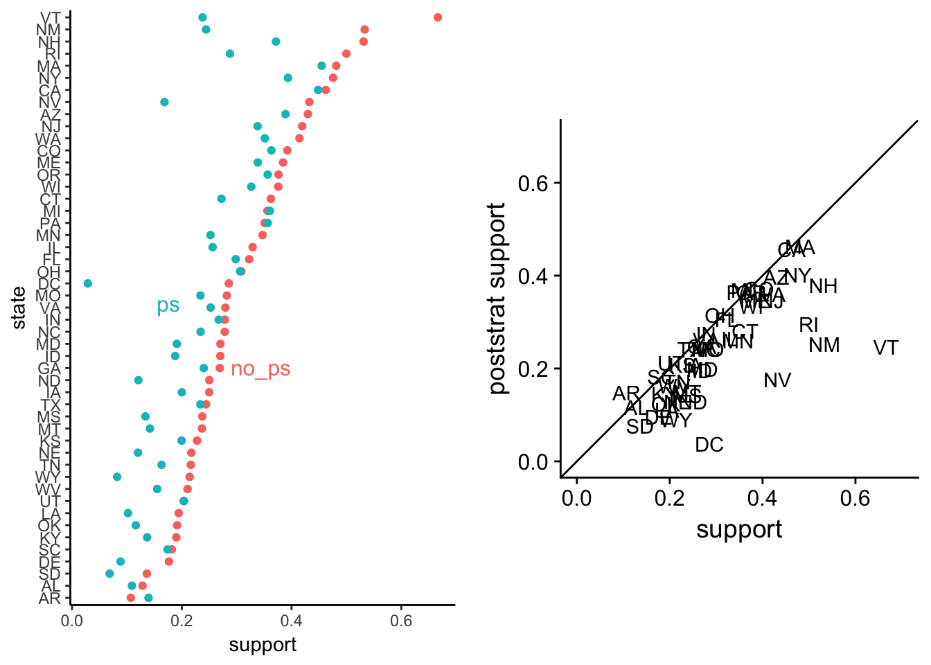
The left plot shows a lot of variation between the poststratified averages. The right plot1 indicates that every poststratified state average is pushed near zero. That’s not necessarily a problem in its down right, but we should still debug the model.
Within each state, each group is a certain percentage of the total populations. And the percentages of each group should add up to one, the entire state population:
Census %>%
  group_by(state) %>%
  summarise(percent = sum(cpercent.state)) %>%
  arrange(desc(percent))
## # A tibble: 51 x 2
## state percent
## <chr> <dbl>
## 1 IN 1
## 2 MA 1
## 3 IL 1
## 4 NV 1
## 5 WY 1
## 6 KS 1
## 7 NH 1
## 8 NM 1
## 9 AK 1
## 10 ME 1
## # ... with 41 more rowsWhat’s going own in our model? Let’s look at the total percent of demographic groups included in the survey by each state.
grp.means %>%
  group_by(state) %>%
  summarise(total_percent = sum(cpercent.state, na.rm=TRUE)) %>%
  filter(state != "") %>%
  ggplot(aes(x = state, y = total_percent)) +
  geom_text(aes(label=state), hjust=0.5, vjust=0.25) +
  theme(axis.text.x=element_blank(),
        axis.ticks.x=element_blank()) +
  coord_fixed(ratio=8) + ylim(c(0,1.1))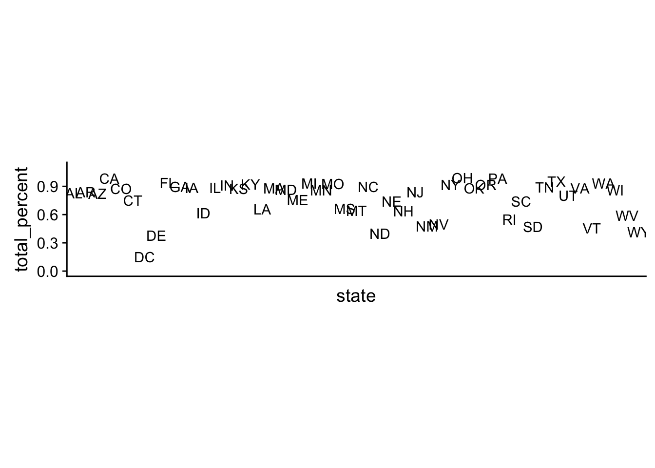
Clearly the survey does not have responses from each demographic group in each state. This lack of data makes poststratifying on the state level uninformative, since there is no subgroup average to make. Implicitly, this model is assuming the missing demographic group’s support is 0%.
But that isn’t a sound model. Let’s take black men for example. Our survey has no responses from black men in South Dakota, but they make up x% of the state. We would be underestimating the level of support in the state by assuming no black men support gay marriage.
However, we do have the responses from black men from neighboring states and all other states around the country. It would be better to use that data to make an informative guess for the level of support black men have in South Dakota. This idea motivates the use of multilevel regression.
Model 2: Maximum Likelihood Multilevel Model
In our disaggrated model, we took the empirical averages for each demographic group sampled in the survey. Within many states, however, not every demographic group was sampled. As described in the previous section, we’d like a way to infer missing demographic groups within each state using the support for the group outside of the state.
The straightforward way to estimate state and demographic group opinions is a regression model, where every factor of a category (states, races, etc.) is allowed to have a unique intercept. In particular, we are going to work with a multilevel regression model. I think that this introduction by the Stan team is a great starting point.
The key idea behind the multilevel model is that the level of support for gay marriage among races, for example, is partially pooled with information from other races. Multilevel regression is a compromise between two extremes:
No pooling: the assumption that each race has a completely independent opinion on gay marriage
Complete pooling: The assumption that all races have the same opinion
The model accomplishes this by allowing each group to have a varying intercept that is sampled from an estimated population distribution of varying intercepts. Our first model will be the maximam likelihood approximation to the full Bayesian model. This is the model Jonathan fits in the MRP Primer, expect I’m removing poll because he doesn’t actually use it to predict opinion.
approx.mod <- glmer(formula = yes.of.all ~ (1|race.female)
                    + (1|age.cat) + (1|edu.cat) + (1|age.edu.cat)
                    + (1|state) + (1|region) +
                    + p.relig + kerry.04,
data=marriage.data, family=binomial(link="logit"))summary(approx.mod)## Generalized linear mixed model fit by maximum likelihood (Laplace
## Approximation) [glmerMod]
## Family: binomial ( logit )
## Formula: yes.of.all ~ (1 | race.female) + (1 | age.cat) + (1 | edu.cat) +
## (1 | age.edu.cat) + (1 | state) + (1 | region) + +p.relig +
## kerry.04
## Data: marriage.data
##
## AIC BIC logLik deviance df.resid
## 7487.8 7548.6 -3734.9 7469.8 6332
##
## Scaled residuals:
## Min 1Q Median 3Q Max
## -1.9534 -0.7108 -0.4848 0.9917 3.9206
##
## Random effects:
## Groups Name Variance Std.Dev.
## state (Intercept) 0.0003689 0.01921
## age.edu.cat (Intercept) 0.0073012 0.08545
## race.female (Intercept) 0.0508921 0.22559
## region (Intercept) 0.0379336 0.19477
## edu.cat (Intercept) 0.1341613 0.36628
## age.cat (Intercept) 0.2930770 0.54137
## Number of obs: 6341, groups:
## state, 49; age.edu.cat, 16; race.female, 6; region, 5; edu.cat, 4; age.cat, 4
##
## Fixed effects:
## Estimate Std. Error z value Pr(>|z|)
## (Intercept) -1.477570 0.525617 -2.811 0.00494 **
## p.relig -0.014754 0.004932 -2.992 0.00277 **
## kerry.04 0.018777 0.006798 2.762 0.00575 **
## ---
## Signif. codes: 0 '***' 0.001 '**' 0.01 '*' 0.05 '.' 0.1 ' ' 1
##
## Correlation of Fixed Effects:
## (Intr) p.relg
## p.relig -0.549
## kerry.04 -0.726 0.652Jonathan manually builds the inverse link function and applies it to every row of the Census data to calculate the estimated state opinion on the state level taking into account each demographic group. I’ll take a different approach here.
The lme4 package provides a method predict to easily make predictions on new data. This is a generic implementation of rebuilding the link function based off of regression coefficients. And if we apply predict to the Census data2, we can also make estimates for groups not sampled in the survey, such as the missing black men in South Dakota we noted above, by applying the estimated black men opinion and the overall state opinion.
Moreover, we can also address other problems in the survey. For example,
marriage.data %>%
  filter(state == "AK", state == "HI")
## [1] state p.evang p.mormon
## [4] kerry.04 poll poll.firm
## [7] poll.year id statenum
## [10] statename region.cat female
## [13] race.wbh edu.cat age.cat
## [16] age.cat6 age.edu.cat6 educ
## [19] age democrat republican
## [22] black hispanic weight
## [25] yes.of.opinion.holders yes.of.all state.initnum
## [28] region no.of.all no.of.opinion.holders
## [31] race.female age.edu.cat p.relig
## <0 rows> (or 0-length row.names)no one from Alaska and Hawaii were included in the survey. But by applying the predict function to the Census, not only can we estimate the opinion by applying the overall state average, but we can also break down the opinion by the percentages of demographic groups within Alaska and Hawaii. This gives a more robust state estimate, and allows for poststratification.
ps.approx.mod <- Census %>%
  mutate(support = predict(approx.mod, newdata=.,
                                allow.new.levels=TRUE, type='response')) %>%
  mutate(support = support * cpercent.state) %>%
  group_by(state) %>%
  summarise(support = sum(support))
We’ll investigate this model further after we build the full Bayesian model.
Model 3: Full Bayesian Model
I am going to fit the full Bayesian modeling using the Stan interface brms. The model specification will be the same as the approximate model in the previous section, except for some weakly informative priors on the standard deviations of the varying intercepts useful for convergence.
bayes.mod <- brm(yes.of.all ~ (1|race.female) + (1|age.cat) + (1|edu.cat)
                 + (1|age.edu.cat) + (1|state) + (1|region)
                 + p.relig + kerry.04,
                 data=marriage.data, family=bernoulli(),
                 prior=c(set_prior("normal(0,0.2)", class='b'),
                         set_prior("normal(0,0.2)", class='sd', group="race.female"),
                         set_prior("normal(0,0.2)", class='sd', group="age.cat"),
                         set_prior("normal(0,0.2)", class='sd', group="edu.cat"),
                         set_prior("normal(0,0.2)", class='sd', group="age.edu.cat"),
                         set_prior("normal(0,0.2)", class='sd', group="state"),
set_prior("normal(0,0.2)", class='sd', group="region")))summary(bayes.mod)## Family: bernoulli
## Links: mu = logit
## Formula: yes.of.all ~ (1 | race.female) + (1 | age.cat) + (1 | edu.cat) + (1 | age.edu.cat) + (1 | state) + (1 | region) + p.relig + kerry.04
## Data: marriage.data (Number of observations: 6341)
## Samples: 4 chains, each with iter = 2000; warmup = 1000; thin = 1;
## total post-warmup samples = 4000
## ICs: LOO = NA; WAIC = NA; R2 = NA
##
## Group-Level Effects:
## ~age.cat (Number of levels: 4)
## Estimate Est.Error l-95% CI u-95% CI Eff.Sample Rhat
## sd(Intercept) 0.41 0.09 0.26 0.62 4000 1.00
##
## ~age.edu.cat (Number of levels: 16)
## Estimate Est.Error l-95% CI u-95% CI Eff.Sample Rhat
## sd(Intercept) 0.10 0.06 0.01 0.25 1433 1.00
##
## ~edu.cat (Number of levels: 4)
## Estimate Est.Error l-95% CI u-95% CI Eff.Sample Rhat
## sd(Intercept) 0.32 0.09 0.18 0.52 4000 1.00
##
## ~race.female (Number of levels: 6)
## Estimate Est.Error l-95% CI u-95% CI Eff.Sample Rhat
## sd(Intercept) 0.23 0.08 0.12 0.41 4000 1.00
##
## ~region (Number of levels: 5)
## Estimate Est.Error l-95% CI u-95% CI Eff.Sample Rhat
## sd(Intercept) 0.22 0.09 0.09 0.42 4000 1.00
##
## ~state (Number of levels: 49)
## Estimate Est.Error l-95% CI u-95% CI Eff.Sample Rhat
## sd(Intercept) 0.06 0.04 0.00 0.15 1626 1.00
##
## Population-Level Effects:
## Estimate Est.Error l-95% CI u-95% CI Eff.Sample Rhat
## Intercept -1.48 0.52 -2.50 -0.47 4000 1.00
## p.relig -0.01 0.01 -0.02 -0.00 4000 1.00
## kerry.04 0.02 0.01 0.00 0.03 4000 1.00
##
## Samples were drawn using sampling(NUTS). For each parameter, Eff.Sample
## is a crude measure of effective sample size, and Rhat is the potential
## scale reduction factor on split chains (at convergence, Rhat = 1).So what are the advantages to the full Bayesian model? The most obvious benefit is the total accounting of uncertainty in the model. For example, let’s take a look at the standard deviation of group-level intercepts:
library(tidybayes)

approx_sd <- broom::tidy(approx.mod) %>%
  filter(stringr::str_detect(term, "sd_"))

bayes.mod %>%
  gather_samples(`sd_.*`, regex=TRUE) %>%
  ungroup() %>%
  mutate(group = stringr::str_replace_all(term, c("sd_" = "","__Intercept"=""))) %>%
  ggplot(aes(y=group, x = estimate)) +
  ggridges::geom_density_ridges(aes(height=..density..),
                                rel_min_height = 0.01, stat = "density",
                                scale=1.5) +
  geom_point(data=approx_sd)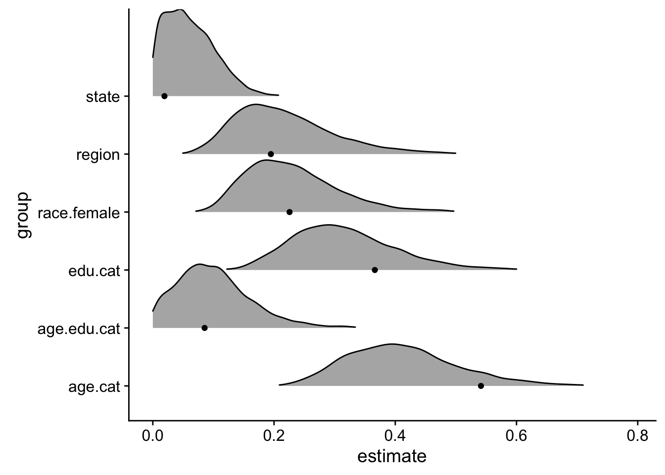
The Bayesian model provides a distribution of all possible standard deviations that the varying intercepts could be sampled from, while the approximate model only provides a single point estimate3. Moreover, that point estimate does not necessarily reflect the mean of the distributions. In general, point approximates cannot quantify uncertainty and are more likely to overfit the data4.
But first, let’s compute the point estimate for the level of state support for gay marriage and poststratify. As in the approximate model, we want to fit this model on the Census data.
ps.bayes.mod <- bayes.mod %>%
  add_predicted_samples(newdata=Census, allow_new_levels=TRUE) %>%
  rename(support = pred) %>%
  mean_qi() %>%
  mutate(support = support * cpercent.state) %>%
  group_by(state) %>%
  summarise(support = sum(support))
In the next section, we’ll compare all three models using point estimates and we’ll work to include uncertainty from the Bayesian model.
Model Comparisons
Using the comparison scatterplots, we can easily see the changes between each model.
mod.disag[nrow(mod.disag) + 1,] = list("AK", mean(mod.disag$support), "no_ps")
mod.disag[nrow(mod.disag) + 1,] = list("HI", mean(mod.disag$support), "no_ps")

disag.approx <- bind_cols(mod.disag, ps.approx.mod) %>% compare_scat() +
  xlab("disag model") + ylab("approx mod")
disag.bayes <- bind_cols(mod.disag, ps.bayes.mod) %>% compare_scat() +
  xlab("disag model") + ylab("bayes model")
approx.bayes <- bind_cols(ps.approx.mod, ps.bayes.mod) %>% compare_scat() +
  xlab("approx model") + ylab("bayes model")

plot_grid(disag.approx, disag.bayes, approx.bayes)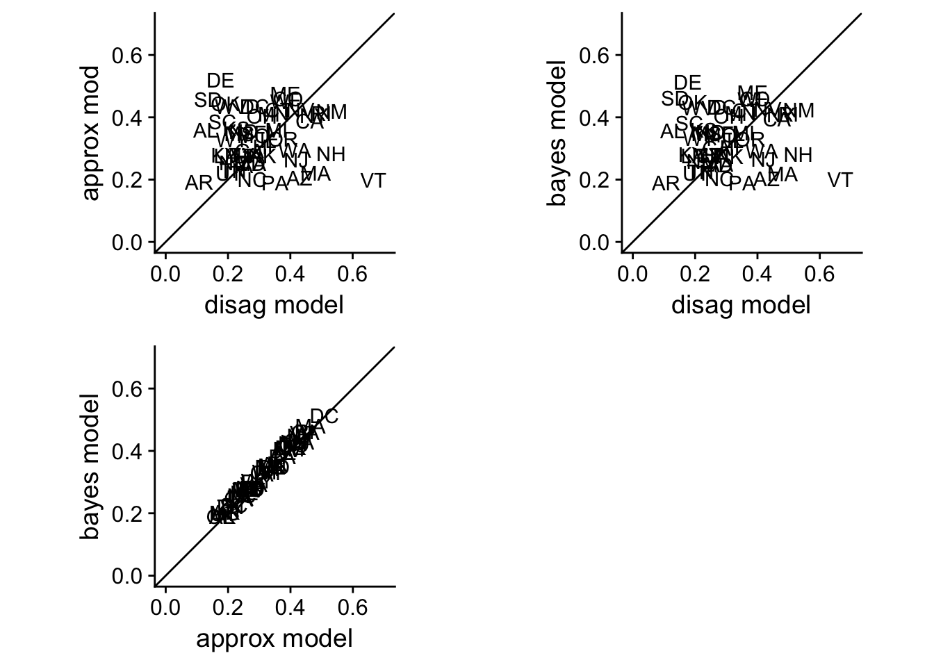
Although the parameter values differed between the approximate and the full Bayesian model, the predictions are near identical.
However, the point estimate in the Bayesian model doesn’t take full advantage of the posterior distribution brms and Stan calculate. For that, we can sample the posterior distribution for the entire census data 500 times and see the distribution of poststratified support for gay marriage within each state.
str(predict(bayes.mod, newdata=Census, allow_new_levels=TRUE,
        nsamples=500, summary=FALSE))
## int [1:500, 1:4896] 1 0 0 0 1 1 0 1 0 0 ...bayes.mod %>%
add_predicted_samples(newdata=Census, allow_new_levels=TRUE, n=500)## # A tibble: 2,448,000 x 19
## # Groups: state, p.evang, p.mormon, kerry.04, crace.WBH, age.cat,
## # edu.cat, cfemale, .freq, cfreq.state, cpercent.state, region,
## # race.female, age.edu.cat, p.relig, .row [4,896]
## state p.evang p.mormon kerry.04 crace.WBH age.cat edu.cat cfemale .freq
## <chr> <dbl> <dbl> <dbl> <int> <int> <int> <int> <int>
## 1 AK 12.44 3.003126 35.5 1 1 1 0 467
## 2 AK 12.44 3.003126 35.5 1 1 1 0 467
## 3 AK 12.44 3.003126 35.5 1 1 1 0 467
## 4 AK 12.44 3.003126 35.5 1 1 1 0 467
## 5 AK 12.44 3.003126 35.5 1 1 1 0 467
## 6 AK 12.44 3.003126 35.5 1 1 1 0 467
## 7 AK 12.44 3.003126 35.5 1 1 1 0 467
## 8 AK 12.44 3.003126 35.5 1 1 1 0 467
## 9 AK 12.44 3.003126 35.5 1 1 1 0 467
## 10 AK 12.44 3.003126 35.5 1 1 1 0 467
## # ... with 2,447,990 more rows, and 10 more variables: cfreq.state <dbl>,
## # cpercent.state <dbl>, region <chr>, race.female <dbl>,
## # age.edu.cat <dbl>, p.relig <dbl>, .row <int>, .chain <int>,
## # .iteration <int>, pred <int> # rename(support = pred) %>%
# mutate(support = support * cpercent.state) %>%
# group_by(.iteration, add = TRUE) %>%
# mean_qi()# bayes.pred %>%
# ggplot(aes(y=state, x=support)) +
# ggridges::geom_density_ridges(aes(height=..density..),
# rel_min_height = 0.01, stat = "density",
# scale=1)The idea for this plot comes from Matt Vuorre, who called them with-subject scatterplots in his blog post. Austin Rochford also uses a similar chart in his MRP Prime walkthrough. And I am using the two letter state abbreviation labels instead of points as Gelman recommends.↩
By design the Census provides every combination of demographic groups within each state. If that wasn’t the case, I would enter in each unique demographic and state factor into
modelr::data_grid, which would automiatcally generate every possible combination of results. This is a very useful tool.↩Technically, we could calculate the standard error from the approximate model. However, it may not be accurate and it is computationally expensive. It took me way longer to calculate the standard error via bootstrapping compared to fitting the full Bayesian model in
brms.↩Check out this article for a nice discussion in the context of machine learning.↩